About Our Data

Sources of Champions TumorGraft® Models

Champions Oncology has several sources for the clinically-relevant TumorGraft (patient-derived xenograft (PDX)) models it maintains in its bank. The first source is from the work we do directly with patients in which we develop TumorGraft models from individual patient tumors and use them to help guide treatment decisions in the clinic. The second source of Champions TumorGraft® models in our bank is research collaborations we have established with external institutes and hospitals. We are also obtaining a large number of new and drug discovery-relevant models through clinical validation studies being led by our Medical Affairs team. Additionally, we will be adding to our tumor bank through a series of co-clinical initiatives and matched patient clinical programs. We will keep you informed of these initiatives as they progress.

In summary, Champions Oncology remains committed to building the world’s most clinically-relevant TumorGraft model bank.

Model Status (Availability of TumorGraft Models)

Model status provides information on how readily clients may access models for use in their studies; it is defined across three categories:

Established - sufficient model inventory is available in liquid nitrogen, ready for immediate use.
Banking - TumorGraft material is being generated for storage in liquid nitrogen. Models under this designation may be available for use depending on how much material has already been banked (early or late stage banking).
Engrafted - a new tumor that has recently been implanted into recipient animals is showing definitive signs of growth. Champions TumorGraft® models in this category are normally transitioned to Banking after tumor material starts being generated and stored in liquid nitrogen. This process takes approximately 2-3 months.

Patient/Tumor Profile and Patient Treatment

Tumor Profile

This is information related to the tumor that was collected from a patient to develop a TumorGraft model (pathological and histological determinants). We also include the Champions TumorGraft (CTG) number, which is a unique identifier assigned to each TumorGraft model by our Model Development and Characterization team. Information that may in any way allow identification of patients (name, date of birth etc.) is not available though this database and is restricted to only those individuals at Champions Oncology who are rigorously trained in safe-guarding patient confidentiality. Finally, all patients who donate samples to generate TumorGraft models are required to sign an Informed Consent document.

CTG Number	Unique identification number given to TumorGraft models.
Tumor Type	Defines the type of cancer the patient was diagnosed with.
Tumor Status	Classifies the harvested tumor as a primary or metastatic lesion.
Tumor Subtype sarcoma, glioma, head & neck models only	Defines the subtype of tumor the patient was diagnosed with.
ER/PR/HER2 Status breast models only	Specifies if the estrogen, progesterone, or HER2 receptors are expressed.
Harvest Site	Identifies the site in the body where the tumor was harvested from.
Histology	Indicates what the tumor looks like under a microscope.
Tumor Grade	Defines how closely the tumor resembles normal tissue.

Much of this information comes to us from pathology reports or from clinical updates given by the treating oncologist. We are also in the process of reviewing the histology and grade of Champions TumorGraft® models (based on H&E stained slides we have generated) with the help of our pathologist consultant team.

As noted in the table above, data for breast, sarcoma, glioma, and head & neck Champions TumorGraft®models is slightly modified to contain more information specifically related to these tumor types. For breast models we include whether the estrogen, progesterone, and HER2 receptors are expressed in the models (identified from patient pathology reports), whilst for sarcoma, glioma, and head & neck models, Tumor Subtype is included.

Patient Profile

This information relates to data about the patient from whom the tumor was obtained. It includes:

Diagnosis	First diagnosis or Recurrent tumor.
Treatment History	Pretreated (therapy received before Champions TumorGraft® model development) or Naïve.
Disease Stage	I-IV, based on radiology/pathology reports.
BRCA1/2 status breast and ovarian models only	Mutated, Deleted, or Normal.
Smoking History	Smoker, Former smoker, Non-smoker.
Age	In years, at time of tumor resection.
Gender	Male or Female.
Ethnicity	Caucasian, Black or African American, Asian, Hispanic, Mixed, Native Hawaiian or Pacific Islander.

Please note that although Patient Profile and Tumor Profile are described separately here, they are grouped together in the same table in the database.

Patient Treatment

This is information related to the treatments a patient received before and after the collection of their tumor.

CTG Number	Unique identification number given to TumorGraft models.
Pre/Post-Collection	Indicates whether a treatment was received before or after collection of the tumor.
Drug	Identifies the generic name of the drug received by the patient.
Outcome	Defines the response of the patient to the drug (Responded, No response, Mixed response, N/A (neoadjuvant)) (based on radiology screens/blood tests).
Duration (months)	Indicates how long the patient responded to the drug.

Please note that for Mixed or No response, the length of response is not included because some level of disease progression has occurred. These tables only include chemotherapy drugs (labeled using generic drug names). We do not show radiotherapy treatments or alternative/experimental therapies (e.g. naturopathy or experimental vaccines). We also obtain primary radiological and blood test records that help define treatment responses. Many of the post-collection treatments are identified by Champions Oncology through our work directly with patients (see above).

Champions TumorGraft® Model Growth Curves

One important parameter for Champions TumorGraft® models is their growth pattern. Our bioinformatics specialist has gathered all the accumulated growth data we have for every model and performed a linear regression analysis of this data in order to generate a mean growth curve for each model (depicted as Days versus Mean tumor volume in mm3). We also show a 95% confidence interval for each data point, represented as purple shading around the curve, to give an estimate of the uncertainty in the analysis.

Growth Characteristics

Doubling Time	17 days
150mm3	46 days
1000mm3	93 days

Some growth metrics based on this analysis are also provided to help users evaluate the growth pattern of each model. These are the average time (in days) it has taken each model to reach either 150mm3 or 1000mm3 following implantation of a single tumor fragment with a volume of 64mm3 into the flank of a recipient mouse.

Champions TumorGraft® Drug Sensitivity (Drugs Tested)

One of the pre-eminent features of our Champions TumorGraft® Database is the availability of information on the response of our TumorGraft models to different chemotherapeutic agents. The general scheme for screening drugs against our TumorGraft models is shown in the figure below. Tumor fragments (around 64mm3) are implanted into the flanks of recipient mice and tumor dimensions are recorded with digital calipers. Estimated tumor volumes are calculated using the formula: TV= width2 x length x π/2. Once tumor implants reach a volume of approximately 200mm3, dosing with test agents (or vehicle control) begins (designated as Day 0). Test agents are administered according to instructions from the manufacturer, as well as established literature. Tumor dimensions are measured as indicated previously and data, including individual and mean estimated tumor volumes (Mean TV ± SD), recorded for each group.

At study completion, percent tumor growth inhibition (%TGI) values are calculated for all test agents (T) versus the vehicle control (C) using initial (i) and final (f) tumor measurements by the formula: %TGI=[1-(Tf-Ti)/(Cf-Ci)]x100.

At present, we are only showing tables with the %TGI values for each test agent screened against each model in the database. We are not currently showing drug response curves. We are in the process of re-analyzing all of the drug response data for each model using more rigorous algorithms in a similar fashion to our growth curves. These drug response curves will be made available in subsequent updates to our database.

Molecular Characterization

The Champions TumorGraft® database provides molecular profiles for models through Next Generation Sequencing (NGS) technology and immunohistochemical staining of model tissue. At the present time these profiles include data on:

Gene Mutations (SNVs and indels)	from Whole Exome Sequencing
Copy Number Variations (CNV)	from Whole Exome Sequencing
Gene Splice Variants	from RNASeq
Gene Expression Levels	from RNASeq
Gene Fusions and Translocations	from RNASeq
Protein Expression	Label-Free Data-Independent Acquisition (DIA) Quantitative Proteomics
Tumor Pathology	from H&E staining of models

Champions Oncology has established collaborations with the New York Genome Center, Rutgers University, and the Broad Institute to generate the NGS data for its TumorGraft models. All initial processing of data is performed at these centers, with final annotation and packaging for display undertaken by bioinformaticists at Champions. As well as showing this information in the database, processed NGS data files can also be downloaded by clients from individual model pages using the provided hyperlinks (where available).

RNA sequencing

Sequencing

RNA sequencing libraries are prepared using the TruSeq Stranded mRNA Library Preparation Kit in accordance with the manufacturer’s instructions. Briefly, 500ng of total RNA is used for purification and fragmentation of mRNA. Purified mRNA undergoes first and second strand cDNA synthesis and cDNA is then adenylated, ligated to Illumina sequencing adapters, and amplified by PCR (using 10 cycles). Final libraries are quality-controlled using fluorescent-based assays including PicoGreen (Life Technologies) or Qubit Fluorometer (Invitrogen) and Fragment Analyzer (Advanced Analytics) or BioAnalyzer (Agilent 2100), prior to sequencing on an Illumina HiSeq2500 sequencer (v4 chemistry) using 2 x 50bp cycles.

Expression Analysis

After sequencing, FASTQ files are aligned to a combined index of human and mouse reference genomes and all reads mapping uniquely to mouse removed (a process called “de-mousing”). The resultant demoused FASTQ files are then aligned to the NCBI GRCh37 human reference using STAR aligner (v2.4.2a) (PMID: 23104886). Quantification of genes annotated in Gencode v19 is performed using FeatureCounts (v1.4.3) and quantification of transcripts using RSEM (doi: 10.1186/1471-2105-12-323). QC collected with Picard (v1.83) and RSeQC (PMID: 22743226; http://broadinstitute.github.io/picard/). Normalization of feature counts is done using the edgeR package (doi:10.1093/bioinformatics/btp616).

Fusion Analysis

Fusion analysis is applied to raw FASTQ files using FusionCatcher (http://dx.doi.org/10.1101/011650) using the most updated human genome references.

Common Questions About RNASeq Metrics And Features

1. What does RPKM stand for and how is it calculated? RPKM values are a normalized measure of how abundantly expressed a specific gene is. RPKM stands for Reads Per Kilobase Million and is calculated from the number of reads (sequenced fragments) that align to a reference human genome (see above). These absolute read counts need to be corrected for gene length (the “Per Kilobase” part of RPKM) and sample sequencing depth (the “Million” part of RPKM) because these two elements can artificially skew higher the absolute reads for some genes. Long genes will naturally have more reads aligning to them because they have more fragments that can be sequenced. Samples with greater sequencing depth will have more reads aligning to them because more of the fragmented mRNA (cDNA) is actually sequenced.

In simple terms, RPKM is calculated as follows:

1. The total number of reads for an RNA sequencing run (i.e. the total number of RNA/cDNA fragments that were sequenced) is divided that number by 1,000,000 to give a "Million” scaling factor.
1. The total number of reads for a gene in a model (i.e. how many sequences corresponded to our gene of interest) is divided by the "million scaling factor". This is an RPM value. This helps normalize for the sequencing depth or put more simply, how well a gene in a model was able to be sequenced versus that gene in other models. If a sequencing run in one model happened to work better, you will naturally get more reads out the other end which may artificially make it look as if a gene is expressed more highly than it really is.
1. The RPM value is divided by the total length of the exons (in kilobases) to give you RPKM. This normalizes for gene length because longer genes will have more reads associated with them. Without doing this, it may artificially make it look as if they are more highly expressed than other genes.
1. Why is it Log2(RPKM+1)? The range of values for RPKM can be quite large, giving a non-normal distribution and making downstream analyses more difficult. A log transformation (log2) is applied, which makes the RPKM values distribute more normally (along the archetypal bell curve). Because there can be a lot of genes that are not expressed or below the level of detection, many RPKM values are 0. This leads to an error when you try to log transform (Logs cannot be calculated for 0 values). To avoid this, a value of 1 is added to ALL the RPKM values before the log transformation. This is the Log (RPKM+1) column in the data sheet.
1. Expression data is usually measured relative to normal tissue, is this also done at Champions? We do not have a matched normal against which to measure how much more or less a gene is expressed in our tumor models. As an in silico substitute, the mean of the Log2(RPKM+1) for a gene across ALL models is taken and used as a "cancer-normal" baseline (because across so many different cancer types and models, the gene is assumed to be over AND under-expressed, overall yielding something approximating normal). This is what the Log2(RPKM+1) value for a gene in a model is measured against in order to obtain fold expression. We also calculate the standard deviation for these mean Log2(RPKM+1) values for each gene.
  Clients should note that because the mean Log2(RPKM+1) for a gene is calculated from across ALL samples in our RNASeq dataset, these values are likely to change slightly for each gene as we add more sequenced models to our dataset i.e. we re-evaluate the mean Log2(RPKM+1) values for each gene when we add more sequenced models to our RNASeq dataset.

2. How are z-scores calculated? Z-scores are one way to measure the expression of a gene in one model relative to all models. They are a measure of the number of standard deviations away from the mean Log2(RPKM+1) for a gene in a specific model is. They are calculated by subtracting the mean Log2(RPKM+1) for a gene from the Log2(RPKM+1) value for that gene in the model of interest and dividing the result by the standard deviation of the Log2(RPKM+1) values for that gene.

3. How is fold expression calculated? Fold expression is another metric that measures the expression of a gene in a model relative to the mean expression of that gene across all models (using our “cancer-normal” substitute, mean Log2(RPKM+1)). In essence, it is calculated by dividing the Log2(RPKM+1) value for a specific gene in a specific model by the mean Log2(RPKM+1) value for that gene. However, there are additional correction factors that go into the calculation to account for batch sequencing effects (correcting for differences in Log2(RPKM+1) values that can be attributed to samples being sequenced at different times across different runs).

Proteomics Data

Proteomics and Phosphoproteomics

Peptide intensities were obtained by Spectronaut. Protein intensities were calculated by MSstats, using quantile-normalization per sample. Outliers were detected and removed using Median Absolute Deviation (MAD), with a cutoff of median +/- 3MADs. The values shown are Variance Stabilizing Normalization (VSN) - normalized and imputed abundances (log2(intensities)).

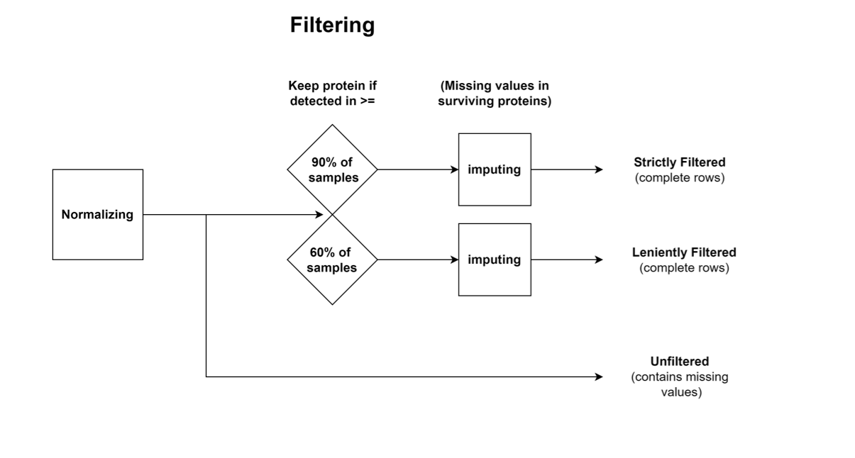
Three datasets are provided for proteomics/phosphoproteomics, which were generated by different processing steps after normalization:
1. Strictly Filtered: Contains only proteins which were detected in >= 90% of the samples, constituting a conservative dataset; The missing values were imputed.

2. Leniently Filtered: Contains only proteins which were detected in >= 60% of the samples, constituting a lenient dataset; The missing values were imputed.

3. Unfiltered: Values with neither filtering nor imputation.

For "missing at random" proteins: bpca- Bayesian PCA missing value estimation
For "missing not at random" proteins (e.g. low/undetected in many samples): MinProb - imputation of left-censored missing data by random draws from a Gaussian distribution centered in a minimal value.

Kinase Data

Kinase activity scores were calculated from phospho-peptide abundances using the ssGSEA algorithm, based on an assembly of databases containing kinase → substrate links information (Signor, PhosphositePlus, Hijazi et al. 2020).

Please Note: Proteomics Data is normalized per indication whereas Champions PDX Data is normalized based on the whole bank.

Whole exome sequencing (WES)

Whole Exome Sequencing is performed as paired-end 125-bp reads using an Illumina HiSeq 2500 machine following the manufacturer’s protocol using a defined capture kit (usually Agilent v4XT, but also V4Target, SureSelectTarget, and SeqCap EZ exome v3) to reach an average coverage of 100x. Raw reads from each model are aligned to a concatenated human and mouse reference genomes (GRC37/hg19 and GRCm38/mm10 respectively) using BWA aligner followed by filtering out of reads not aligning to the human contigs ("de-mousing").

Indel/SNP Analysis

Local realignment around INDELs and base quality score recalibration is done using the GATK pipeline. SNP analysis is conducted using multiple callers (muTect, Lofreq and Strelka) against a normal cell line sample as a control (NA12878). SNPs below the quality threshold (quality score <20, Read depth <10) are removed from the analysis, as are SNPs found in online germline databases (HapMap, ExAC, 1000G).

CNV Analysis

Copy Number Variation Analysis is performed using EXCAVATOR (10.1186/gb-2013-14-10-r120) with the NA12878 normal cell line as a baseline control.