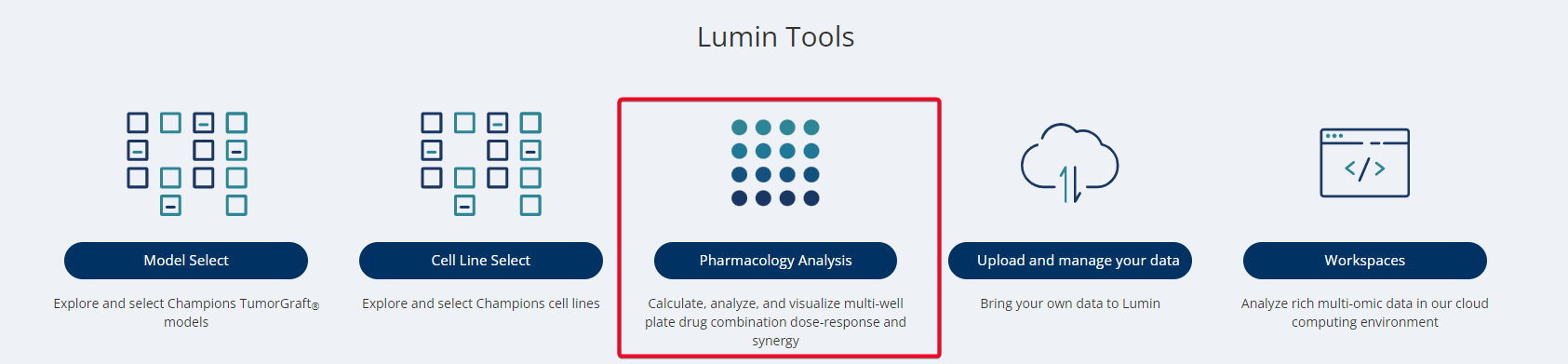
Pharmacology Analysis
Calculate, analyze, and visualize multi-well plate drug combination dose response and synergy.
General Description
Our Pharmacology Analysis tool aims to allow users to upload plate maps from drug response studies to compute IC50 values and create dose-response curves, and also analyze your combination studies by uploading data to simultaneously perform Loewe, Bliss, ZIP or HSA measurements of synergy, additivity or antagonism. Synergy results are presented as a table, heat map and 3D surface plot.
You can collaborate with colleagues by sharing your data files. Please Note: This is not an automatic feature, you need to check a box first to make the analysis visible to your company.
Starting an Analysis

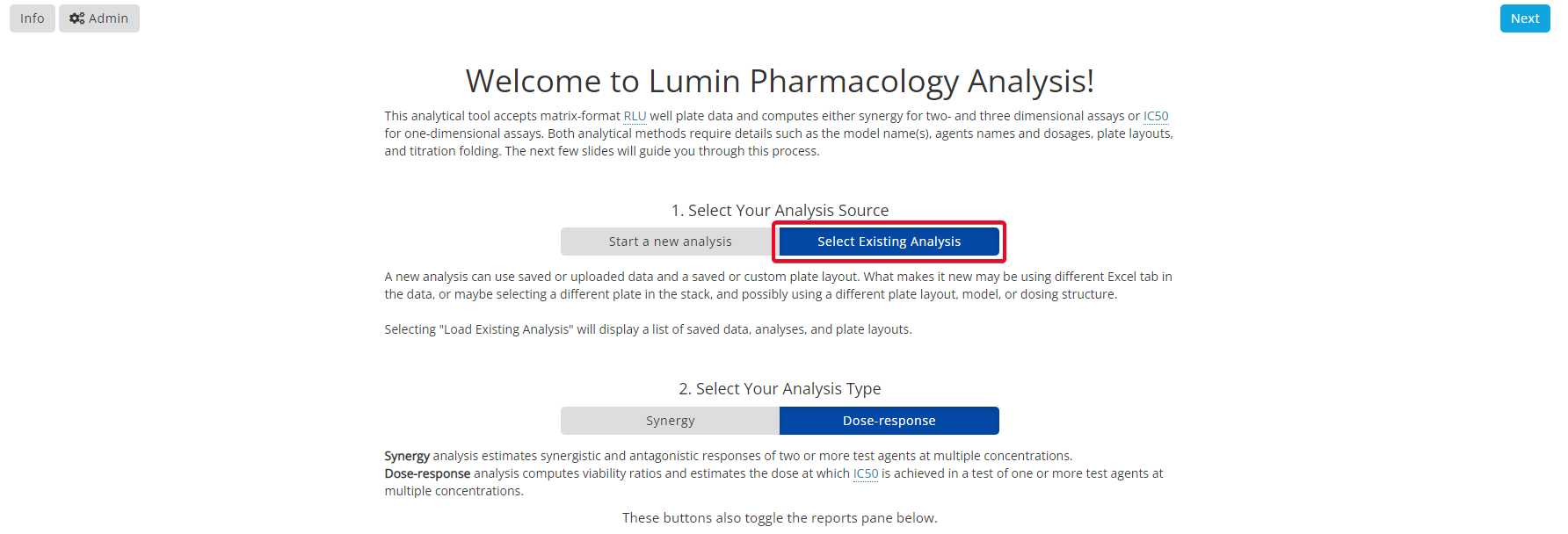
Step 1: Introduction and Analysis Type
- Select Your Analysis Source. Select either 'Start a New analysis' or 'Load Existing Analysis' depending on whether you have previously uploaded data into the Pharmacology Analysis tool or not.
- Select Your Analysis Type. Choose between 'Synergy Analysis' or 'Dose-Response Analysis'.
- Next. Click to move to the next step.
- Info. Overview for using the Lumin Pharmacology Analysis Tool.
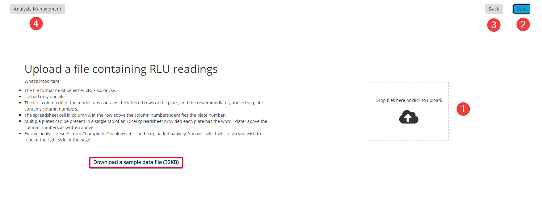
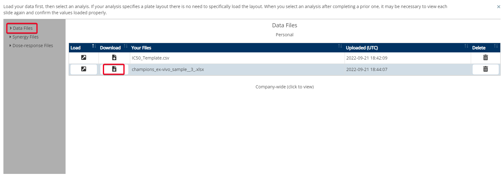
Step 2: Upload File
- Upload File. Either drag and drop your file to the cloud icon or click to browse and upload your file. Please Note: All uploaded files are stored for future use but can be removed after completing an analysis using the "Analysis Management" button.
- Next. Click to move to the next step.
- Back. Click to go to the previous step.
- Analysis Management. Shows both personal and company-wide data files saved to your Lumin account.
You can also download a sample file by clicking the text that is highlighted in the red box above.
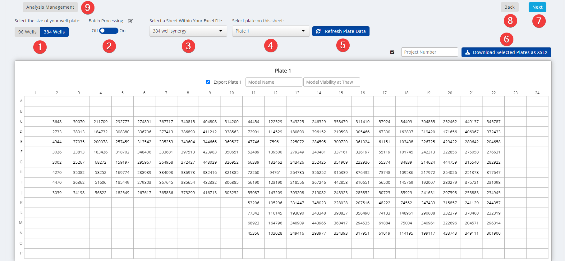
Step 3: Select Plate
- Select the Size of Your Well Plate. Choose between 96 wells or 384 wells.
- Batch Processing. Off for single plate analysis. On to apply the layout and parameters to all sheets of the file or all plates of the sheet. Use the editor button to select which sheets or plates to include.
- Select a Sheet Within Your Excel File. Select which plate you would like to analyse from the dropdown menu.
- Select a Plate to Analyze. Select a plate to analyze individually. Please Note: For Synergy Analysis, if there are duplicate plates you can select 'Average All Plates'.
- Refresh Plate Data After changing any of the parameters please click 'Refresh Plate Data' to update this.
- Download Selected Plates. You can download the selected plates as XSLX by entering a project number in the input box and clicking the download button.
- Next. Click to move to the next step.
- Back. Click to go to the previous step.
- Analysis Management. Shows both personal and company-wide data files saved to your Lumin account.
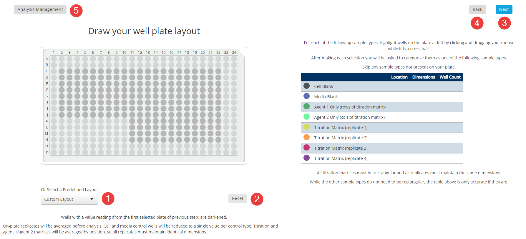
Step 4: Plate Layout
- Select a Layout. Either create a custom layout by selecting wells individually and categorizing them or choose a predefined layout from the dropdown menu.
- Reset. Reset the plate layout to default where wells with data are dark grey and wells with no data are light grey.
- Next. Click to move to the next step.
- Back. Click to go to the previous step.
- Analysis Management. Shows both personal and company-wide data files saved to your Lumin account.
Synergy Analysis Input

Synergy Step 5: Plate Titration
- Identify Titration Folding. Fill in all blank text boxes with relevant information from your data file or enter concentrations manually. Please Note: Hovering your mouse over the 'i' will give you information on each input.
- Next. Click to move to the next step.
- Back. Click to go to the previous step.
- Analysis Management. Shows both personal and company-wide data files saved to your Lumin account.

Synergy Step 6: Analysis Parameters
- Select an Analysis Method. Choose between the 4 analysis methods in the dropdown menu or select 'All' to do all 4 analysis methods. Please Note: Description on each method can be found in the image above or in 'Key Terms' below.
- Next. Click to move to the next step.
- Back. Click to go to the previous step.
- Analysis Management. Shows both personal and company-wide data files saved to your Lumin account.

Synergy Step 7: Results & Report
- Visualization. View results from each analysis as either a 3D surface plot or heatmap. You can also toggle between the upper and lower confidence intervals or the mean. Please Note: Surface plots are semi-interactive. Click and move around to show points of synergy, additivity and antagonism.
- Data. View data as Response, Synergy or in downloadable Table format.
- Next. Click to move to the next step.
- Back. Click to go to the previous step.
- Analysis Management. Shows both personal and company-wide data files saved to your Lumin account.

Synergy Step 8: Save
- Model/Agent/Dosage And Analysis Parameters. Enter a 'Name' and 'Description' for the analysis data you are saving. Select the '-' dropdown to save the plate layout separately.
- Save. Once all information is entered correctly click the 'Save' button. Please Note: Check box to make the analysis visible to your company.
- Back. Click to go to the previous step.
- Analysis Management. Shows both personal and company-wide data files saved to your Lumin account.
Syngery Analysis Interpretation
The summary synergy scores can be interpreted as the average excess response due to drug interactions (i.e. synergy score of 15 corresponds to 15% of response beyond expectation). There is no particular threshold to define a good synergy score, since combination synergy is highly context-specific. However, based on our experience, the synergy scores near 0 gives limited confidence on antagonism or synergy. So when a synergy score is:
- Less than -10: the interaction between two drugs is likely to be antagonistic;
- From -10 to 10: the interaction between two drugs is likely to be additive;
- Larger than 10: the interaction between two drugs is likely to be synergistic.
Similar thresholds can be applied to the most synergistic area (MSA) score, which represents the most synergistic 3-by-3 dose-window in a dose-response matrix.
Dose Response Analysis Input

Dose Response Step 5: Plate Titration
- Identify Titration Folding. Fill in all blank text boxes with relevant information from your data file or enter concentrations manually. Each test block can be labeled with a test model and a test agent with individual statistical fitting parameters. Parameters include the top and bottom fitted values, the set of negative control wells against which the test wells are normalized (default is all but a subset of them can be defined in the plate layout if more than one negative control is present on the plate), and if the test agent is a combination of two or more agents an alternative set of reference wells can be identified which will be used when fitting the model. Please Note: Hovering your mouse over the 'i' will give you information on each input.
- Next. Click to move to the next step.
- Back. Click to go to the previous step.
- Analysis Management. Shows both personal and company-wide data files saved to your Lumin account.

Dose Response Step 6: Analysis Parameters
- Parameterize Your Analysis. For most analyses you can accept the default values without issue. They include "Day 0 Background" and "Raw Data Day 0" values which can be entered as either space or comma separated values and when supplied appear on the QC barplot for the plate. The "Untreated Well Selection" can be set to use either all negative control wells, the N nearest wells, or a random subset of wells. If anything other than all is selected N can be specified. Please Note: Hovering your mouse over the 'i' will give you information on each input.
- Next. Click to move to the next step.
- Back. Click to go to the previous step.
- Analysis Management. Shows both personal and company-wide data files saved to your Lumin account.

Dose Response Step 7: Results & Report
- Visualization. View data as Response (shown in image) or in downloadable Table format. Outliers Selection Tab shows boxplots of the raw RLU data after background subtraction. Readings flagged as outliers by Grubbs's test are colored bright red. Any outlier point can be excluded from the analysis by clicking it in the plot, then using the "Back" button to revisit the "Parameterize your analysis" page. There you check the box labeled "Remove selected outliers" and click "Next" to return to the refreshed analysis which has now removed the outliers. Report Results Tab allows you to create a PDF report with results from one or many plates, and it also allows you to export IC50 estimates to the "Target & Biomarker Discovery" module.
- Next. Click to move to the next step.
- Back. Click to go to the previous step.
- Analysis Management. Shows both personal and company-wide data files saved to your Lumin account.

Dose Response Step 8: Save
- Model/Agent/Dosage And Analysis Parameters. Enter a 'Name' and 'Description' for the analysis data you are saving. Select the '-' dropdown to save the plate layout separately.
- Save. Once all information is entered correctly click the 'Save' button. Please Note: Check box to make the analysis visible to your company.
- Back. Click to go to the previous step.
- Analysis Management. Shows both personal and company-wide data files saved to your Lumin account.
Under The Hood: Calculating IC50 and Synergy
Many people who use the Lumin dose response calculator have performed similar analyses in Graphpad Prism and are curious to know how our IC50 values compare to those computed in Prism, or they have actually done a comparison and are attempting to explain the difference between the two sets of results. During development and testing we have done our best to "tune" Lumin to produce similar results as Prism where possible. This is possible because both Prism and the Lumin Pharmacology analysis tool fit a fairly well-documented 4-parameter log-logistic model (LL.4).
How IC50 values are computed
Prior to fitting the LL.4 Lumin removes the background luminance by subtracting the mean media control reading from each observation. It then computes the viability ratio relative to the control as observed/vehicle control. The viability ratios are then moved to model fitting.
The model fitting in Lumin is done by the software program R using the drc package (see reference below). The 4 parameters in the model are the bottom, the top, the slope, and the IC50. In Lumin the default is to fix the bottom at 0 and the top at 1, although it is possible to unset these and have the model fit them in addition to the IC50 and the slope. Lumin also uses a mean-least-squares estimation method and the default starting functions for the optimization method, but it is possible to override the start values for both IC50 and slope if necessary. Beyond the option to unfix the bottom and/or top and set start values, the only other deviation from the drc defaults is to set the optimization method to "Nelder-Mead" rather than "BFGS", as we have observed this method produces output that match Prism to 4 significant figures. Lumin also has a configurable default of 1000 maximum iterations.
When we observe a difference between Lumin and Prism it is usually due to higher than ideal variance in the data. In these cases, the stochastic nature of the optimization algorithm leaves the door open for two optimization methods to converge at slightly different IC50 estimates within acceptable relative tolerance, due either to using different relative tolerance values or to using different hop sizes that may permit them to identify different local minimum fit estimators rather than a single global minimum. The default value for relative convergence in drc is 1e-7, and the dose-scaling and response-scaling thresholds are both set to 1e-15. The following table lists the default optimization and LL.4 model settings for Lumin and Prism.
| Parameter | Lumin | Prism |
|---|---|---|
| Bottom | 0* | 0* |
| Top | 1* | 1* |
| IC50 start | automatic* | automatic* |
| Slope start | automatic* | automatic* |
| Regression method | non-robust mean least squares | non-robust least squares* |
| Convergence criteria | 1e-7 | Medium/strict* |
| Maximum iterations | 1000* | 1000* |
| Outlier test | Grubbs | Grubbs/ROUT* |
| Optimization method | Nelder-Mead | Marquardt |
*User configurable
How Synergy is computed
Two and three-agent synergy calculations are done in R using the package synergyfinder. This package is exceptionally well documented by the authors (see references below), and Lumin users should refer to that documentation for descriptions of the methods. Prior to passing the observed values to synergyfinder, Lumin pre-processes the data by subtracting the mean background reading (the media control wells) from each observed value, then it computes the percent inhibition as 1 - observed/vehicle control. All synergy estimations are based on the inhibition metric.
How to Download
Select the 'Pharmacology Analysis' Tool from the Lumin Homepage.
Under “2. Select Your Analysis Type”, choose Dose Response. Your report(s) will be listed underneath Dose-response Reports at the bottom of the screen, click the download button to export the PDF.

To download the raw RLU values, on the same page, select 'Load Existing Analysis'. Then select 'Data Files' on the left hand side menu. Next, select the data file(s) to download.
Key Terms
Loewe defines the expected effect as if a drug was combined with itself. Unlike the HSA and the Bliss independence models, which give a point estimate using different assumptions, the Loewe additivity model evaluates the dose-response curves of individual drugs using a nonlinear solver.
The Bliss model assumes two agents exert their effects independently, and the expected combined effect can be calculated based on the monotherapy effect of combined agent 1 and agent 2.
Zero Interaction Potency (ZIP) calculates the expected effect of two drugs under the assumption that they do not potentiate each other. The statistical analysis for synergy scores of the whole dose-response matrix is estimated under the null hypothesis of non-interaction (zero synergy score).
Highest Single Agent (HSA) states that the expected combination effect equals the higher effect of the individual agents.
Grubbs's Test - This is a test used to detect outliers in a univariate data set assumed to come from a normally distributed population (also known as the Maximum Normed Residual Test).
References and Acknowledgements
Synergy Analysis is based on the work of Zheng et al: Zheng, S.; Wang, W.; Aldahdooh, J.; Malyutina, A.; Shadbahr, T.; Pessia, A.; Jing, T. SynergyFinder Plus: towards a better interpretation and annotation of drug combination screening datasets. bioRxiv 2021.06.01.446564 (2021) doi:10.1101/2021.06.01.446564
Synergy Analysis Interpretation is based on the (SynergyFinder - Documentation, 2022): Synergyfinder.fimm.fi. 2022. SynergyFinder - Documentation. [online] Available at: https://synergyfinder.fimm.fi/synergy/synfin_docs/ [Accessed 2022].
Dose-Response Analysis is based on the work of Ritz et al: Ritz C, Baty F, Streibig JC, Gerhard D (2015) Dose-Response Analysis Using R. PLoS ONE 10(12): e0146021. doi:10.1371/journal.pone.0146021 or http://journals.plos.org/plosone/article?id=10.1371/journal.pone.0146021
Updated over 2 years ago